Understanding the Knapsack Problem: From Theory to Everyday Use

The Knapsack Problem is more than a math puzzle; it’s a lens through which we view resource allocation in logistics, finance, and even diet planning. Imagine you’re packing a backpack for a hike: you have limited space, and you want to maximize the value of the items you bring. That simple scenario mirrors a problem that has challenged computer scientists and operations researchers for decades.

What Is the Knapsack Problem?

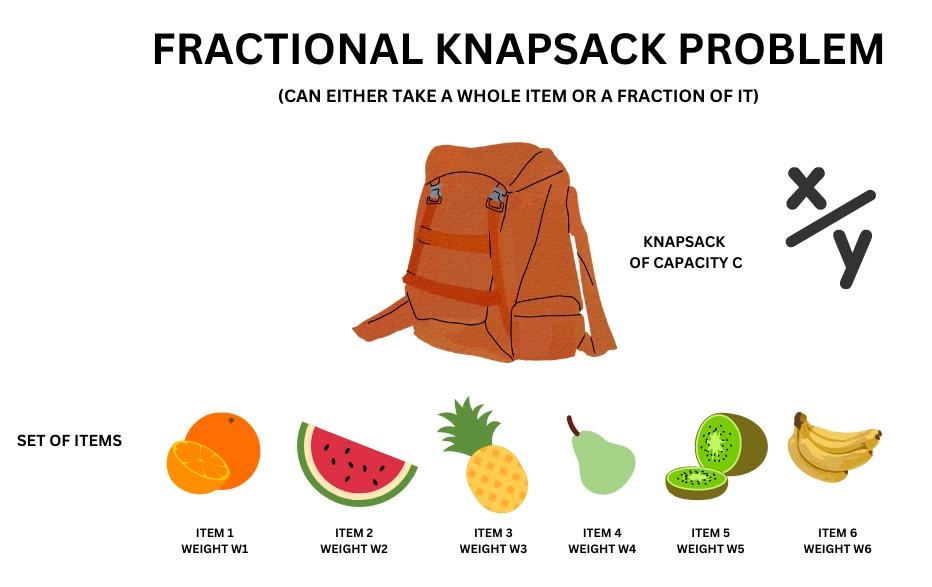
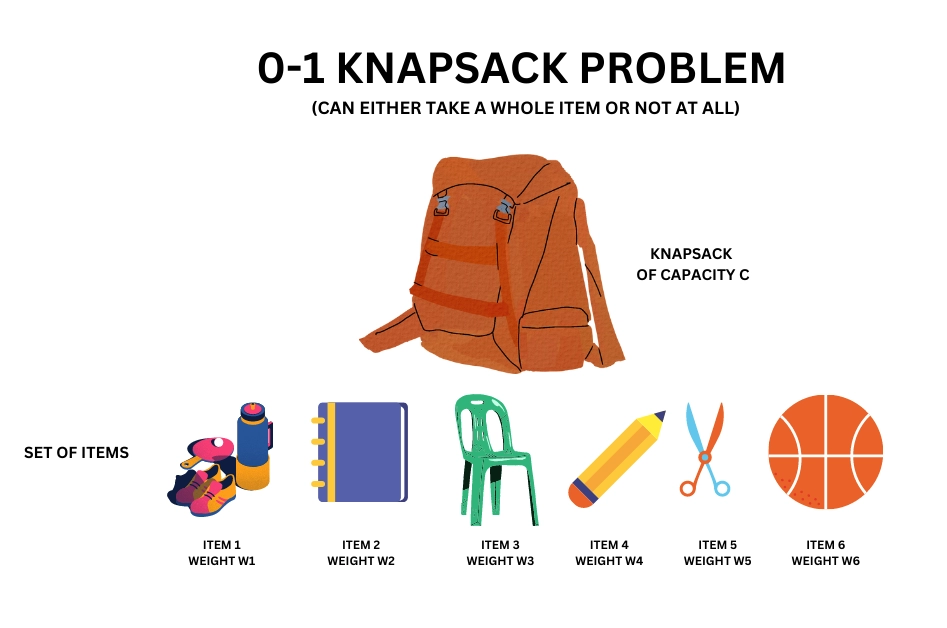
At its core, the problem asks: given a set of items, each with a weight and a value, how do you choose a subset that fits within a weight limit while maximizing total value? The classic version—called the 0/1 Knapsack—requires that each item be taken whole or not at all. The fractional variant allows you to split items, which is useful when items are divisible, like liquid or bulk goods.

Real-World Applications

While the name conjures images of backpacks, the knapsack framework pops up everywhere:

• Budget planning: Selecting projects to fund under a fixed capital constraint.
• Cargo loading: Deciding which cargo pieces to ship when weight limits are strict.
• Advertising: Choosing ad slots that fit a time budget while maximizing revenue.
• Data compression: Packing the most valuable data chunks into limited storage.

Each scenario boils down to balancing weight against value—literal or figurative.

Why It’s Computationally Hard

The 0/1 Knapsack Problem is NP‑complete, meaning that as the number of items grows, the time required to find the exact best solution can explode exponentially. In practice, exact algorithms are viable for hundreds or thousands of items, but for tens of thousands or millions, you’ll need approximations or heuristics.

Dynamic Programming Approach

The most common exact algorithm uses dynamic programming (DP). Think of it as building a table where each row represents an item and each column represents a possible weight capacity. The entry in the table stores the maximum value achievable with that capacity using the items considered so far. The recurrence is simple:

DP[i][w] = max(DP[i-1][w], DP[i-1][w‑weight_i] + value_i)

Here, DP[i-1][w] is the value when you skip item i, and DP[i-1][w‑weight_i] + value_i is the value when you include it. By iterating through all items and capacities, you eventually fill the table, and the bottom‑right cell gives the optimal value. The DP solution runs in O(n·W) time, where n is the number of items and W the capacity, which is acceptable when W is moderate.

Greedy Approximation for the Fractional Variant

When items can be divided, a greedy strategy works beautifully. Sort items by value‑to‑weight ratio, then pick as much as possible from the highest ratio until the knapsack is full. This method guarantees an optimal solution for the fractional problem in linearithmic time, O(n log n), thanks to the sorting step.

When to Choose Which Strategy

Decide based on your constraints:

• Exact, small‑scale problem: Use dynamic programming.
• Large scale or real‑time decision: Greedy or a heuristic like a genetic algorithm.
• Mixed constraints (e.g., multiple resource limits): Extend DP to multi‑dimensional variants or resort to linear programming relaxations.

Common Mistakes to Avoid

Even seasoned practitioners trip over subtle pitfalls:

• Ignoring the weight constraint: Adding an item that exceeds the capacity and then backtracking is inefficient.
• Assuming value is the sole factor: A high‑value item with a massive weight might reduce overall benefit.
• Overcomplicating the DP table with unnecessary dimensions, which bloats memory usage.

Extending the Concept: Multi‑Knapsack and Knapsack with Dependencies

Real problems often involve multiple containers or dependencies between items. The multi‑knapsack problem places items into several bags, each with its own capacity. The knapsack with dependencies adds constraints like “if item A is chosen, item B must also be selected.” These richer models require more sophisticated algorithms, often combining DP with branch‑and‑bound or integer programming.

Practical Tips for Implementing the DP Solution

1. Use a 1‑D array: Instead of a full 2‑D table, iterate items in reverse weight order to reuse the same array, halving memory.
2. Cap the weight dimension: If the maximum weight is huge, consider scaling or using a value‑based DP to limit table size.
3. Track item selection: Store decisions separately if you need the actual items, not just the total value.
4. Profile early: Small test cases can reveal hidden loops or index errors before scaling up.

Frequently Asked Questions

• What is the difference between 0/1 Knapsack and Fractional Knapsack? The 0/1 version forces whole items; the fractional version allows splitting items, which changes the algorithmic approach.
• Can the knapsack algorithm handle negative values? Standard formulations assume non‑negative values; negative values usually indicate items that cost resources without adding benefit.
• Is there a closed‑form solution? For the fractional variant, yes—greedy sorting suffices. For 0/1, no closed form exists; you need exhaustive or approximate methods.
• How does the knapsack problem relate to the subset‑sum problem? Subset‑sum is a special case where all values equal weights, turning the goal into exactly filling the capacity.