Mastering Simpson’s Rule: A Simple Guide to Numerical Integration
What Simpson’s Rule Actually Does
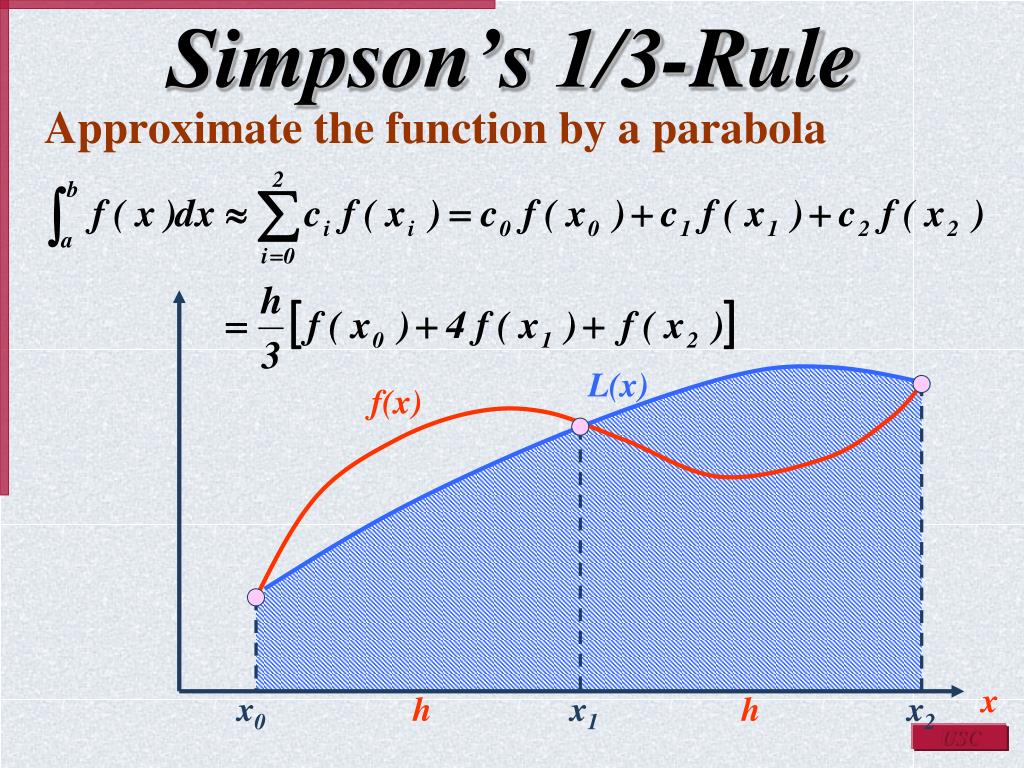
When you need the area under a curve but the antiderivative is messy—or outright unavailable—numerical integration steps in. Among the many techniques, Simpson’s rule stands out for its blend of simplicity and accuracy. In essence, it replaces a segment of a function with a parabola, then adds up the little parabolic slices to approximate the total integral. Because a quadratic curve can capture the curvature of smooth functions better than a straight line, the error drops dramatically compared to the basic trapezoidal rule.
Deriving the Classic Formula
Imagine you have three equally spaced points: a, m = (a+b)/2, and b. You fit a second‑degree polynomial P(x) through the values f(a), f(m), and f(b). Integrating P(x) from a to b yields the familiar one‑panel Simpson’s rule:
(b‑a) / 6 · [ f(a) + 4 f(m) + f(b) ]
For a longer interval you simply split the domain into an even number n of subintervals, each of width h = (b‑a)/n, and apply the one‑panel formula repeatedly. The composite version looks like this:
(h/3) · [ f(x₀) + 4 ∑f(x₂k‑1) + 2 ∑f(x₂k) + f(xₙ) ]
where the odd‑indexed sum runs over the interior points with odd indices, and the even‑indexed sum runs over those with even indices (excluding the endpoints).
When to Reach for Simpson’s Rule
Not every integral benefits equally from Simpson’s approach. Here are a few tell‑tale signs that the method will serve you well:
- The integrand is smooth—no sudden jumps or sharp corners.
- You can afford an even number of subintervals; the rule relies on pairing intervals.
- High accuracy is desired but you don’t want to venture into high‑order Gaussian quadrature.
If the function wiggles wildly or contains singularities, other strategies—like adaptive quadrature—might be safer.
Common Pitfalls and How to Dodge Them
Even a straightforward technique can trip you up if you overlook the details. Below are the most frequent mistakes and quick fixes.
- Uneven spacing: Simpson’s rule assumes equally spaced nodes. If your data points are irregular, either interpolate onto a uniform grid or switch to a method that tolerates uneven spacing.
- Odd number of panels: The composite rule needs an even n. If you accidentally choose an odd count, simply add one more subinterval; the extra work is minimal.
- Ignoring the error term: The theoretical error is proportional to h⁴ · f⁽⁴⁾(ξ) for some ξ in the interval. In practice, halving the step size usually shrinks the error by about 16×, which is a handy sanity check.
A Quick Worked Example
Let’s approximate the integral of sin x from 0 to π. Analytically the answer is 2, but we’ll see how Simpson’s rule gets us there.
Choose n = 4 subintervals, so h = (π‑0)/4 = π/4. The nodes are 0, π/4, π/2, 3π/4, and π. Their sine values are 0, √2/2, 1, √2/2, and 0 respectively.
Plugging into the composite formula:
(h/3) · [ 0 + 4(√2/2 + √2/2) + 2·1 + 0 ] = (π/12) · [ 0 + 4√2 + 2 ] ≈ (π/12)·(7.656) ≈ 2.00
The result matches the exact value to two decimal places, illustrating why Simpson’s rule is often called “the sweet spot” between simplicity and precision.
Tips for Efficient Implementation
If you’re coding this up, a few practical tricks can keep things tidy.
- Pre‑compute the factor h/3 once, then reuse it.
- Separate the odd‑index and even‑index sums; a single loop with a modulus check does the job cleanly.
- Validate that n is even before starting—throw an informative error otherwise.
In languages like Python, a vectorized approach with NumPy can reduce the loop entirely, while in C or Java a straightforward for‑loop is usually fast enough for modest n.
FAQ
Is Simpson’s rule better than the trapezoidal rule?
Generally yes, provided the function is smooth. Simpson’s rule’s error term involves h⁴ versus the trapezoidal rule’s h², meaning it converges faster as you refine the mesh.
Can I use Simpson’s rule for improper integrals?
Only with caution. If the integrand approaches infinity or oscillates infinitely near an endpoint, you’ll need to transform the integral (e.g., via substitution) or adopt an adaptive method designed for singularities.
How many subintervals are enough?
There’s no one‑size‑fits‑all answer. A good practice is to start with a modest even n (say 8), compute the estimate, then double n and compare. When the change falls below your tolerance, you’ve likely hit a sweet spot.
What if my data points are only available at irregular intervals?
Simpson’s rule assumes uniform spacing, so you’d either resample the data onto a uniform grid (using interpolation) or choose a different quadrature rule like the Romberg method that accommodates uneven nodes.