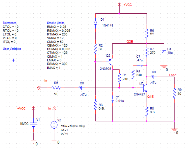
Mastering Monte Carlo Circuit Simulation with IIHSpice: Your Step‑by‑Step Guide

When designers push components to their limits, small variations in temperature, tolerance, or manufacturing can ripple into large performance swings. Monte Carlo simulation in circuit design tackles this uncertainty head‑on by generating thousands of random parameter sets and evaluating how each one affects the outcome. If you’re looking to bring that rigor into your workflow, the IIHSpice Monte Carlo engine is a powerful ally. In this guide we walk through why you need it, how to set it up, and best practices to interpret the results.

Why Use Monte Carlo in Circuit Design?

Physical components are never perfectly identical. Resistors drift by ±1 % or more, capacitors lose a few percent of their value over time, and semiconductor characteristics shift with temperature. Monte Carlo lets you quantify the spread of your design’s performance envelope, revealing margins, worst‑case scenarios, and probabilistic reliability. It’s especially useful for high‑frequency RF circuits, analog front‑ends, and power stages where small variations can cause ripple‑to‑noise, phase error, or even outright failure.

Getting Started with IIHSpice Monte Carlo

IIHSpice provides an intuitive interface to set up and run Monte Carlo studies. Below is a quick checklist for a typical workflow.

Step 1 – Define the Base Circuit

Begin with a standard schematic and SPICE netlist. Ensure all component models are sourced from the library and have the PARAM directives that expose their tolerances. For example:

• R1 n1 n2 R1val=10k @R1_TOL=1%
• C1 n2 n3 C1val=100p @C1_TOL=5%

These directives tell the simulator which parameters to vary.

Step 2 – Activate Monte Carlo

In the IIHSpice GUI, navigate to the “Simulation” tab, select “Monte Carlo,” and choose the number of runs. A good starting point is 1,000 runs for simple analog blocks and 10,000 for high‑precision RF sections. If you prefer a command‑line approach, add:

• .MC N=1000

to the netlist.

Step 3 – Configure Parameter Distributions

IIHSpice allows Gaussian, uniform, or custom distributions. Specify mean and standard deviation for each parameter. If a component’s tolerance is ±5 % but you suspect a tighter manufacturing process, set the standard deviation accordingly. For exotic components, you can import a CSV table that contains measured values.

Step 4 – Run and Export

Hit “Run” and let IIHSpice generate the random instances. The simulation output is a statistical table: mean, standard deviation, min, max, and percentile data for every node voltage, current, and frequency metric you requested. Export this to CSV or use the built‑in histogram viewer.

Practical Tips for Accurate Monte Carlo Analysis

• Choose the right number of runs. Too few runs give a misleading picture; too many waste time. Rule of thumb: 1,000 for exploratory work, 10,000 for final verification.
• Validate your distributions. Compare the simulated spread against measured data from a test batch to ensure the model reflects reality.
• Check convergence. If the standard deviation of a key metric changes drastically between 5,000 and 10,000 runs, you may need more iterations or a refined model.
• Use guard bands. Add safety margins to critical nodes so that even the 99th‑percentile worst case stays within spec.

Interpreting Statistical Outputs

The output table contains several columns:

• Mean – the expected value.
• StdDev – how much the result typically deviates.
• Min/Max – the absolute bounds.
• 95% Confidence – the range that covers almost all runs.

For most design decisions, focus on the 95% confidence interval. If your spec requires a voltage to stay within 5 mV, and the 95% interval spans 8 mV, the design fails the test.

Advanced Features and Troubleshooting

IIHSpice includes features that go beyond basic Monte Carlo.

• Parameter Correlation. If two components share a batch process, you can link their tolerances so they vary together.
• Hybrid Analyses. Combine Monte Carlo with DC sweep or transient analysis to capture dynamic behavior under variation.
• Parallel Execution. Distribute runs across multiple cores or machines to cut simulation time.

Common pitfalls include:

• Over‑specifying tolerances leading to unrealistic spread.
• Neglecting to reset the parameter table between runs.
• Interpreting min/max as absolute worst cases when the underlying distribution is non‑normal.

Case Study: A Simple RC Low‑Pass Filter

Let’s apply Monte Carlo to a 1 kHz RC low‑pass filter. The target cutoff frequency is 1 kHz with ±5 % tolerance. Using IIHSpice, we set:

• R = 1kΩ ±1 %