Isoquant and Isocost Curves: What Every Economist Should Know

When you hear “Isoquant and Isocost curves,” you might picture a set of squiggly lines on a blackboard. In reality, those curves are powerful tools that let firms visualize how to combine labor, capital, and other inputs most efficiently. Grasping their shape and interaction helps you answer questions like “Should I hire more machines or more workers?” without resorting to guesswork. Below, we unpack the intuition behind each curve, show how they intersect, and explain what the sweet spot of production really means.

Understanding Isoquant Curves

An isoquant represents every possible combination of two inputs that yields the same output level. Think of it as a contour line on a topographic map, but instead of elevation, the “height” is the quantity of goods produced. The curve is typically convex to the origin, reflecting diminishing marginal rates of technical substitution (MRTS): as you replace labor with capital, each additional unit of capital replaces fewer units of labor.

Why the convex shape? Early on, when labor is abundant, swapping a few workers for a machine can boost output dramatically. As labor becomes scarcer, each extra machine substitutes for less labor, flattening the curve. This curvature tells managers how flexible their production process is—steeper sections signal that a small change in input mix has a big impact on output.

Key properties to remember:

• Downward sloping: More of one input means you need less of the other to keep output constant.
• Never cross: Two isoquants for different output levels cannot intersect; higher output isoquants lie farther from the origin.
• Marginal rate of technical substitution (MRTS): The slope at any point equals the rate at which one input can be traded for the other while holding output steady.

In practice, firms trace isoquants to see how flexible they are when faced with changing input prices or technology upgrades.

The Role of Isocost Curves

While isoquants focus on output, isocost curves focus on cost. An isocost line shows all input combinations that cost the same amount, given the prices of labor (w) and capital (r). The equation is simple: C = wL + rK, where C is total expenditure, L labor units, and K capital units. Plotting this line on the same graph as the isoquant lets you see which input bundles are affordable.

The slope of an isocost line is –w/r, the negative ratio of input prices. When labor is cheap relative to capital, the line is flatter, indicating you can afford more labor for a given budget. Conversely, an expensive labor market tilts the line steeply, nudging the firm toward capital‑intensive choices.

Isocost curves share two intuitive features:

• Parallelism: With fixed input prices, all isocost lines are parallel; shifting them outward reflects a larger budget.
• Intercepts: The points where the line meets the axes show the maximum amount of one input you could buy if you spent the entire budget on that input alone.

Understanding the slope and intercepts helps managers anticipate how price changes ripple through production decisions.

Combining Isoquants and Isocosts: Finding the Optimal Input Mix

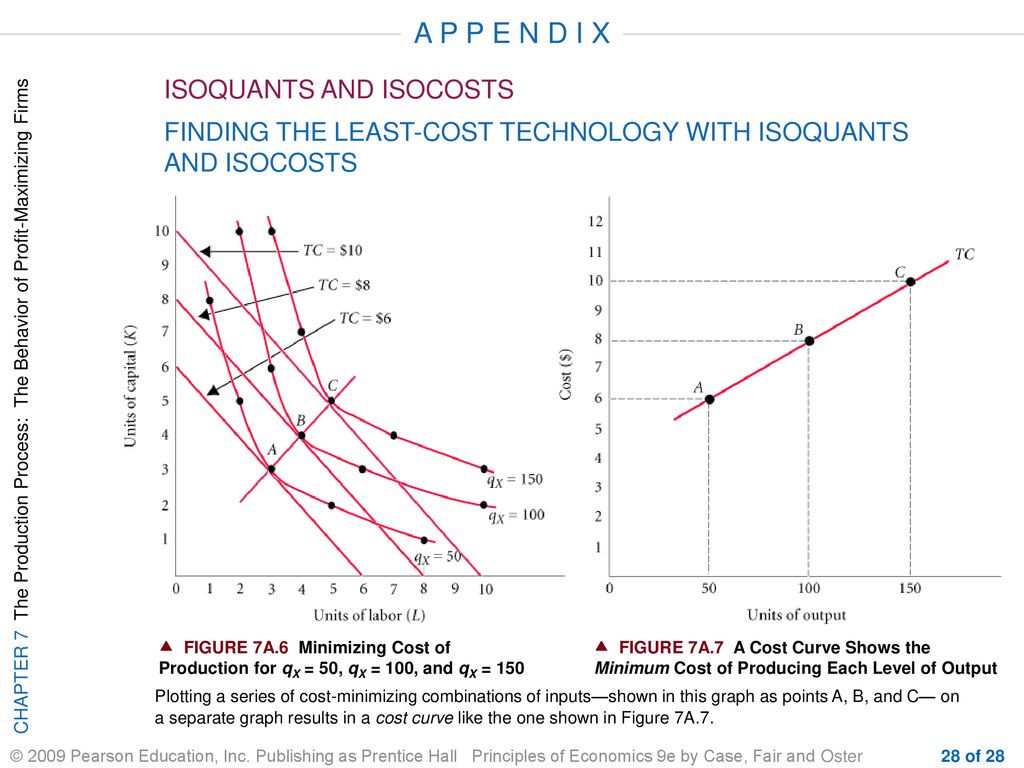
The magic happens where an isoquant just touches an isocost line—tangency. At that point, the firm is producing a given output at the lowest possible cost, or equivalently, achieving the highest output for a given budget. Mathematically, tangency means the slopes are equal:

MRTS = w/r

In plain English, the rate at which the firm is willing to substitute labor for capital (driven by technology) matches the market’s rate of substitution (driven by prices). If the isoquant is steeper than the isocost at a certain point, the firm should use more labor; if flatter, more capital.

Consider a small bakery that produces 1,000 loaves daily. Its isoquant for that output might look like a gently curved line. If the wage rate rises, the isocost line pivots, becoming steeper. The new tangency point moves toward more ovens (capital) and fewer bakers (labor), keeping costs in check while still meeting the 1,000‑loaf target.

Real‑world decision‑making rarely stays static. Input prices fluctuate, technology improves, and demand shifts. Each change redraws either the isoquant, the isocost, or both, prompting a new optimal point. Managers who regularly revisit these curves can adapt faster and avoid costly misallocations.

Practical Steps for Managers

• Identify the current prices of labor (w) and capital (r).
• Estimate the production function to sketch the relevant isoquant(s). Empirical data or industry benchmarks often fill this gap.
• Draw the isocost line for the existing budget, then locate the tangency point.
• Re‑evaluate whenever input prices change or a new technology becomes available.

Common Misconceptions

One frequent misunderstanding is treating isoquants like simple “input‑swap” charts. They actually embed diminishing returns, so the substitution rate isn’t constant. Ignoring this curvature can lead to over‑optimistic forecasts about how much you can replace labor with machines.

Another myth is that the lowest‑cost point always lies on the outermost isoquant. In reality, budget constraints may force a firm to settle on a lower‑output isoquant; the goal then shifts to maximizing output within the feasible cost envelope.

Lastly, some think that isoquants and isocosts are only academic tools. In practice, they underpin modern production‑planning software, cost‑benefit analyses, and even AI‑driven optimization engines.

FAQ

What does the slope of an isoquant tell me?

The slope, called the marginal rate of technical substitution (MRTS), indicates how many units of one input you can give up for an extra unit of the other while keeping output unchanged. A steeper slope means labor is relatively more valuable at that point.

How do changes in input prices affect the optimal input mix?

When the price of labor rises, the isocost line pivots to become steeper, pushing the tangency point toward more capital‑intensive combinations. The opposite occurs when capital becomes cheaper.

Can I use isoquant‑isocost analysis for more than two inputs?

Yes, though the visual representation becomes three‑dimensional or requires advanced software. The core principle—equalizing MRTS with input price ratios—still applies.

Is the tangency point always the best choice?

Under the standard assumptions of profit maximization and continuous, convex production functions, the tangency point yields the lowest cost for a given output. However, real‑world constraints like minimum staffing levels or regulatory caps can shift the feasible region.